star formation simulation in python

1. INTRODUCTION

In this article, we’ll be looking at how to write a star-formation simulation in Python. Sure, the topic may sound intimidating on first glance, but it’s actually pretty straightforward to implement. All you need to know are some basic programming in Python 3 and the fundamentals of vector algebra. An understanding of calculus is a plus, but isn’t absolutely essential. We won’t be deriving equations, but rather using them directly without proof. This article aims to be as beginner-friendly as possible. If you get stuck somewhere, feel free to reach out to me for clarifications.

First things first. What exactly is a simulation? A computer simulation is just a fancy way of saying that we’re using computers to imititate a real-world process. Here, the real world process we’re interested in is that of star formation. In order to imitate the real-world process, we either take a rule-based approach or solve our governing equations. Given that star formation is an actively-studied topic in astrophysics with plenty of equations describing the same, we will be taking the latter approach.

Unlike us, computers can’t work out the solutions to an equation on their own. So, we use different “schemes” to make them solve our governing equations. Here, we’ll be using a technique known as “Smooth Particle Hydrodynamics” in order to solve our equations and run the simulation. The equations are in their vector form.

Given that we’re using Python to solve our equations, we use NumPy to speed up the vector calculations and MatPlotLib to view the simulation results. I will be linking tutorials for the same at the end of the article, and would strongly recommend you check them out to get a better understanding for how these libraries work.

2. FUNDAMENTALS

Before we jump the metaphorical gun and dive head-first into the code, we first need to understand some of the basic concepts that are being used here. Firstly, we’ll look at the physics of how stars form, followed by the simulation technique we’ll be using to visualize the same.

2.1 STAR FORMATION

From our understanding of the sky, we know that outer space is primarily occupied by gas, arbitrarily moving. We also know that stars burn this gas to produce energy, through nuclear fusion. What we’re trying to figure out, is how a gas cloud goes from ungathered motion, to collapsing on itself and starting nuclear fusion.

Broadly speaking, there are 5 major steps in the formation of a star as identified by astronomers. They are as follows:

The initial cloud of molecular gar has only pressure and no gravity. It hence cannot collapse on itself solely by virtue of the motions of its particles
Something (we don’t know what, yet) prompts the gas to form lumps, which in turn leads to gravity dominating over the pre existing pressure.
As these masses of gas aggregate and become heavier, they start rotating and flatten out into a disk (due to moment of Intertia). This disk contains two parts, the accretion disk and the protoplanetary disk.
Continued rotation leads to a stage named “Protostar” that keeps rotating with a positive feedback loop where the more aggregation takes place, the heavier it gets, attracting more clumps.
The accretion disk gets pressurized till the gas starts a fusion reaction. This initial fusion reaction emanates a strong wind through the protoplanetary disc, helping the remaining matter aggregate to form planets and asteroids, while the fusion reaction starts heating up the gas and forms a stable star.

Our simulation will look at a dark cloud, and study how the gravitational collapse occurs. Subsequent steps will require an in-depth understanding of thermodynamics and magnetohydrodynamics, among other things, and are hence beyond the scope of this article. Resources to learn more about this can be found in the resources section.

2.2 Smooth Particle Hydrodynamics

As the name suggests, Smooth Particle Hydrodynamics (SPH) takes a particle-based approach to modelling the properties of a fluid. In our case, we model the clumps of gas as homogenous through interpolation and analytical differentiation. This makes it very simple to apply our standard energy and momentum conservation equations on each “particle”. This is in contrast to traditional fluid dynamics solvers, which make use of meshing and the finite volume approach.

In effect, we study the flow of a fluid by treating it as a collection of particles. We will be looking at how SPH can be implemented in the upcoming sections. For now, this bird’s eye view of SPH is enough to get a feel for what we will be doing.

2.3 GOVERNING EquATIONS

For the SPH simulation, we represent the fluid as a collection of particles. Each particle has an initial position, velocity and mass, with both position and velocity being vectors.

These equations have been adopted from this paper

3. SETUP

Now that we’ve understood the basics of star formation and SPH, we can start making the solver. First, lets import the libraries we’ll be using.

import numpy as np
import matplotlib.pyplot as plt

3.1 Initial Conditions and Constants

Every simulation requires a set of initial conditions to begin with. i.e., the state of the system at t₀. We are defining our initial conditions here. Some of these constants might not make sense just yet, but they will make sense as we move along.

Initially, we start the system with particles (lumps of gas) spread out randomly.

# Constants

N     = 500                   # Number of particles
t     = 0                     # start time of simulation
tEnd  = 8                     # end time for simulation
dt    = 0.01                  # timestep
M     = 2                     # star mass
R     = 0.75                  # star radius
h     = 0.1                   # smoothing length
k     = 0.1                   # equation of state constant
n     = 1                     # polytropic index
nu    = 1                     # damping
m     = M/N                   # single particle mass
lmbda = 2.01                  # lambda for gravity
Nt    = int(np.ceil(tEnd/dt)) # number of timesteps

# Initial Conditions
def initial():
  np.random.seed(42)             # set random number generator seed
  pos   = np.random.randn(N,2)   # randomly selected positions and velocities
  vel   = np.zeros(pos.shape)
  return pos, vel

3.2 KERNEL FUNCTION

As we know, SPH makes use of a smoothening function to distribute the mass of each particle in space. This function uses a kernel function derived from the Dirac δ function. It is essential that the kernel approximates the delta function at its limits to ensure the rest of the math checks out. There are many standard smoothing kernels, like the Gaussian kernel, Cubic spline kernel, Quintic spline kernel, etc. Check this for more info on kernels.

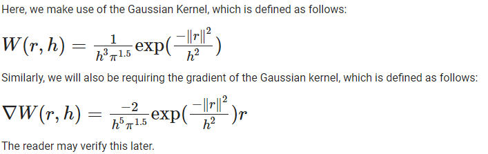
Both of these functions W and ∇W will be used extensively in the following calculations, because discretization helps us shift the gradient onto the kernel. Check this link for more info.

# Gaussian Smoothing Kernel
def kernel(x, y, h):
  """
  Input:
    x : matrix of x positions
    y : matrix of y positions
    h : smoothing length

  Output:
    w : evaluated smoothing function
  """
  # Calculate |r|
  r = np.sqrt(x**2 + y**2)
  # Calculate the value of the smoothing function
  w = (1.0 / (h*np.sqrt(np.pi)))**3 * np.exp( -r**2 / h**2)
  # Return
  return w

# Smoothing Kernel Gradient
def gradKernel(x, y, h):
  """
  Inputs:
    x : matrix of x positions
    y : matrix of y positions
    h : smoothing length

  Outputs:
    wx, wy : the evaluated gradient
  """
  # Calculate |r|
  r = np.sqrt(x**2 + y**2)
  # Calculate the scalar part of the gradient
  n = -2 * np.exp( -r**2 / h**2) / h**5 / (np.pi)**(3/2)
  # Get the vector parts of the gradient
  wx = n * x
  wy = n * y
  # Return the gradient vector
  return wx, wy

3.3 DENSITY CALCULATION

In SPH, the density at a particular point can be found through the formula

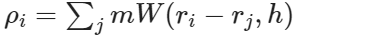
From this formula, we can see that we need to find the distance between all particles to get the density at a particular position. Hence, we can get the density at every position as shown below.

# Solve for the (r_i - r_j) term in the density formula
def magnitude(ri, rj):
  """
  Inputs:
    ri : M x 2 matrix of positions
    rj : N x 2 matrix of positions
  
  Output:
    dx, dy : M x N matrix of separations
  """
  
  M = ri.shape[0]
  N = rj.shape[0]
  
  # get x, y of r_i
  r_i_x = ri[:,0].reshape((M,1))
  r_i_y = ri[:,1].reshape((M,1))
  
  # get x, y of r_j
  r_j_x = rj[:,0].reshape((N,1))
  r_j_y = rj[:,1].reshape((N,1))
  
  # get r_i - r_j
  dx = r_i_x - r_j_x.T
  dy = r_i_y - r_j_y.T
  
  return dx, dy

# Get density at sample points
def density(r, pos, m, h):
  """
  Inputs:
    r   : M x 3 matrix of sampling locations
    pos : N x 3 matrix of particle positions
    m   : particle mass
    h   : smoothing length

  Output:
    rho : M x 1 vector of densities
  """
  
  M = r.shape[0]
  dx, dy = magnitude(r, pos);
  rho = np.sum(m * kernel(dx, dy, h), 1).reshape((M,1))
  
  return rho

3.4 PRESSURE CALCULATION

Since we already have the ρ values from the previous step, we can directly calculate the pressure at each point using the formula

as we had defined in 2.3.

# Find pressure
def pressure(rho, k, n):
  """
  Inputs:
    rho : vector of densities
    k   : equation of state constant
    n   : polytropic index

  Output:
    P : pressure
  """

  P = k * rho**(1+1/n)
  
  return P

3.5 ACCELERATION CALCULATION

In order to track the motion of the particles, we need to know their positions at all time steps. But in order to know the position, we need to know the velocity. And to know the velocity, we require the acceleration of each particle. We can calculate the acceleration acting on each particle at every time step using the following discretization formula:

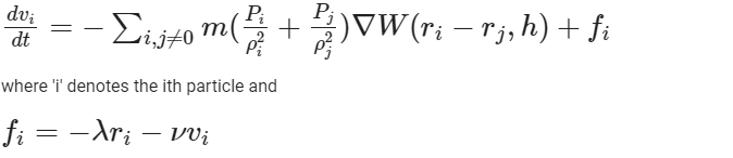
from section 2.3.

Although this formula might look complicated, we can clearly see that it’s just a sum of the components which we had written functions for earlier. Hence, by daisy-chaining the functions, we can evaluate this expression easily.

# Calculate acceleration on particles
def acceleration(pos, vel, m, h, k, n, lmbda, nu):
  """
  Inputs:
    pos   : N x 2 matrix of positions
    vel   : N x 2 matrix of velocities
    m     : particle mass
    h     : smoothing length
    k     : equation of state constant
    n     : polytropic index
    lmbda : external force constant
    nu    : viscosity

  Output:
    a : N x 2 matrix of accelerations
  """
  
  N = pos.shape[0]
  
  # Calculate densities
  rho = density(pos, pos, m, h)
  
  # Get pressures
  P = pressure(rho, k, n)
  
  # Get pairwise distances and gradients
  dx, dy = magnitude(pos, pos)
  dWx, dWy = gradKernel(dx, dy, h)
  
  # Add Pressure contribution to accelerations
  ax = - np.sum(m * (P/rho**2 + P.T/rho.T**2) * dWx, 1).reshape((N,1))
  ay = - np.sum(m * (P/rho**2 + P.T/rho.T**2) * dWy, 1).reshape((N,1))
  
  # Pack acceleration components
  a = np.hstack((ax,ay))
  
  # Add external forces
  a += -lmbda * pos - nu * vel
  
  # Return total acceleration
  return a

4. SIMULATION

Now that the setup is complete, we can move ahead and run the simulation. The simulation requires two main parts. Firstly, we need to set the main loop to run the simulation forward in time. Next, we need to stitch the frames together to form an animation.

4.1 MAIN LOOP

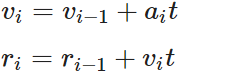
Here, we set up the loop that controls the simulation in the time domain. By tracking the particles in space through time, we can finally tie the simulation together in this loop. Here, we update the velocity and position using Newton’s laws of motion.

import os
import glob
import tqdm

# Creates folder if it doesn't exist
if not os.path.exists('output'):
  os.mkdir('output')
# Else, deletes all images inside it
else:
  files = glob.glob('output/*.png')
  for f in files:
      os.remove(f)

# Disable inline printing to prevent all graphs from being shown
%matplotlib
pos, vel = initial()

# Start loop
for i in tqdm.tqdm(range(Nt)):
  # Update values
  acc = acceleration(pos, vel, m, h, k, n, lmbda, nu)
  vel += acc * dt
  pos += vel * dt
  rho = density(pos, pos, m, h)

  # Plot
  fig, ax = plt.subplots(figsize=(6, 6))

  plt.sca(ax)
  plt.cla()

  # Get color from density
  cval = np.minimum((rho-3)/3,1).flatten()

  # Place particles on map with color
  plt.scatter(pos[:,0],pos[:,1], c=cval, cmap=plt.cm.autumn, s=5, alpha=0.75)

  # Set plot limits and stuff
  ax.set(xlim=(-2.5, 2.5), ylim=(-2.5, 2.5))
  ax.set_aspect('equal', 'box')
  ax.set_facecolor('black')
  ax.set_facecolor((.1,.1,.1))

  # save plot
  plt.savefig(f'output/{i}.png')
  plt.close()

4.2 ANimATION

Now that all the frames are ready, we can stitch them together into a video using OpenCV, and download the simulation.

import cv2

img_array = []

print("Reading Frames")
# List image paths
imgs_list = glob.glob('output/*.png')
lsorted = sorted(imgs_list, key=lambda x: int(os.path.splitext(x[7:])[0]))

for filename in tqdm.tqdm(lsorted):
    img = cv2.imread(filename)
    height, width, layers = img.shape
    size = (width,height)
    img_array.append(img)

out = cv2.VideoWriter('simulation.mp4',cv2.VideoWriter_fourcc(*'MP4V'), 30, size)

# Write to video
print("Writing frames")
for i in tqdm.tqdm(range(len(img_array))):
    out.write(img_array[i])
out.release()

# Download the simulation
from google.colab import files
files.download('simulation.mp4')

5. CONCLUSION AND FUTURE WORK

Through this account, we learnt about how star formation works, and how we can use SPH to simulate the same, albeit in a very crude, 2D case. In the real world, scientists take their simulation results and compare it with observational data, and modify their SPH model assumptions accordingly. Now all that’s left is to go find observational data!

Also, don’t forget to clear the output folder before you re-run simulations!